KO
|
EN
gitlite — search
Search
#python
#artificial-intelligence
#golang
#ai
#cli
#typescript
#containers
#docker
#open-source
#agentic-ai
#pentesting
#rust
gpax
★ 241
Open GitHub ↗
Gaussian Processes for Experimental Sciences
Download README (.md)
Explore Similar Repositories
shogihome
:
PC で動く高機能な将棋の GUI「ShogiHome」の開発リポジトリ
moko-geo
:
Geolocation access for mobile (android & ios) Kotlin Multiplatform development
MyOkHttp
:
对Okhttp3进行二次封装,对外提供了POST请求、GET请求、PATCH请求、PUT请求、DELETE请求、上传文件、下载文件、取消请求、Raw/Json/Gson返回、后台下载管理等功能
presto-hbase-connector
:
presto hbase connector 组件基于Presto Connector接口规范实现,用来给Presto增加查询HBase的功能。相比其他开源版本的HBase Connector,我们的性能要快10到100倍以上。
pydoop
:
A Python MapReduce and HDFS API for Hadoop
// repository documentation
Was this content helpful?
★ 0
(0 ratings)
Select Rating:
★
★
★
★
★
Submit Feedback
Recent Feedback
×
Download README
Do you want to download the
README.md
file for
gpax
?
Download (.md)
# GPax [](https://github.com/ziatdinovmax/gpax/actions/workflows/ci.yml) [](https://github.com/ziatdinovmax/gpax/actions/workflows/notebook_smoke.yml) [](https://codecov.io/gh/ziatdinovmax/gpax) [](https://gpax.readthedocs.io/en/latest/?badge=latest) [](https://badge.fury.io/py/gpax) GPax is a small Python package for physics-based Gaussian processes (GPs) built on top of NumPyro and JAX. Its purpose is to take advantage of prior physical knowledge and different data modalities when using GPs for data reconstruction and active learning. It is a work in progress, and more models will be added in the near future.  ## How to use ### Simple GP #### *1D Example* [](https://colab.research.google.com/github/ziatdinovmax/gpax/blob/main/examples/gpax_simpleGP.ipynb) The code snippet below shows how to use vanilla GP in a fully Bayesian mode. First, we infer GP model parameters from the available training data ```python3 import gpax # Get random number generator keys for training and prediction rng_key, rng_key_predict = gpax.utils.get_keys() # Initialize model gp_model = gpax.ExactGP(1, kernel='RBF') # Run Hamiltonian Monte Carlo to obtain posterior samples for the GP model parameters gp_model.fit(rng_key, X, y) # X and y are numpy arrays with dimensions (n, d) and (n,) ``` In the fully Bayesian mode, we get a pair of predictive mean and covariance for each Hamiltonian Monte Carlo sample containing the GP parameters (in this case, the RBF kernel hyperparameters and model noise). Hence, a prediction on new inputs with a trained GP model returns the center of the mass of all the predictive means (```posterior_mean```) and samples from multivariate normal distributions for all the pairs of predictive means and covariances (```f_samples```). ```python3 posterior_mean, f_samples = gp_model.predict(rng_key_predict, X_test) ``` <img src = "https://user-images.githubusercontent.com/34245227/167945293-8cb5b88a-1f64-4f7d-95ab-26863b90d1e5.jpg" height="60%" width="60%"> For 1-dimensional data, we can plot the GP prediction using the standard approach where the uncertainty in predictions - represented by a standard deviation in ```y_sampled``` - is depicted as a shaded area around the mean value. <img src = "https://user-images.githubusercontent.com/34245227/167945487-05068084-86cb-4104-a792-d39d2f834151.jpg" height="60%" width="60%"> See the full example, including specification of custom GP kernel priors, [here](https://colab.research.google.com/github/ziatdinovmax/gpax/blob/main/examples/gpax_simpleGP.ipynb). #### *Sparse Image Reconstruction* [](https://colab.research.google.com/github/ziatdinovmax/gpax/blob/main/examples/gpax_viGP.ipynb) One can also use GP for sparse image reconstruction. The fully Bayesian GP is typically too slow for this purpose and it makes sense to use a stochastic variational inference approximation (viGP) instead. Code-wise, the usage of viGP in GPax is almost the same as that of the fully Bayesian GP. One difference is that instead of ```num_samples``` we have ```num_steps```. We can also control the learning rate by specifying a ```step_size```. ```python3 # Get training inputs/targets and full image indices from sparse image data X_train, y_train, X_full = gpax.utils.preprocess_sparse_image(sparse_img) # sparse_img is a 2D numpy array # Initialize and train a variational inference GP model gp_model = gpax.viGP(2, kernel='Matern', guide='delta') gp_model.fit(rng_key, X_train, y_train, num_steps=250, step_size=0.05) ``` When we run the ```.predict()``` method, the output is predictive mean and variance computed from a learned single estimate of the GP model parameters: ```python3 y_pred, y_var = gp_model.predict(rng_key_predict, X_full) ``` 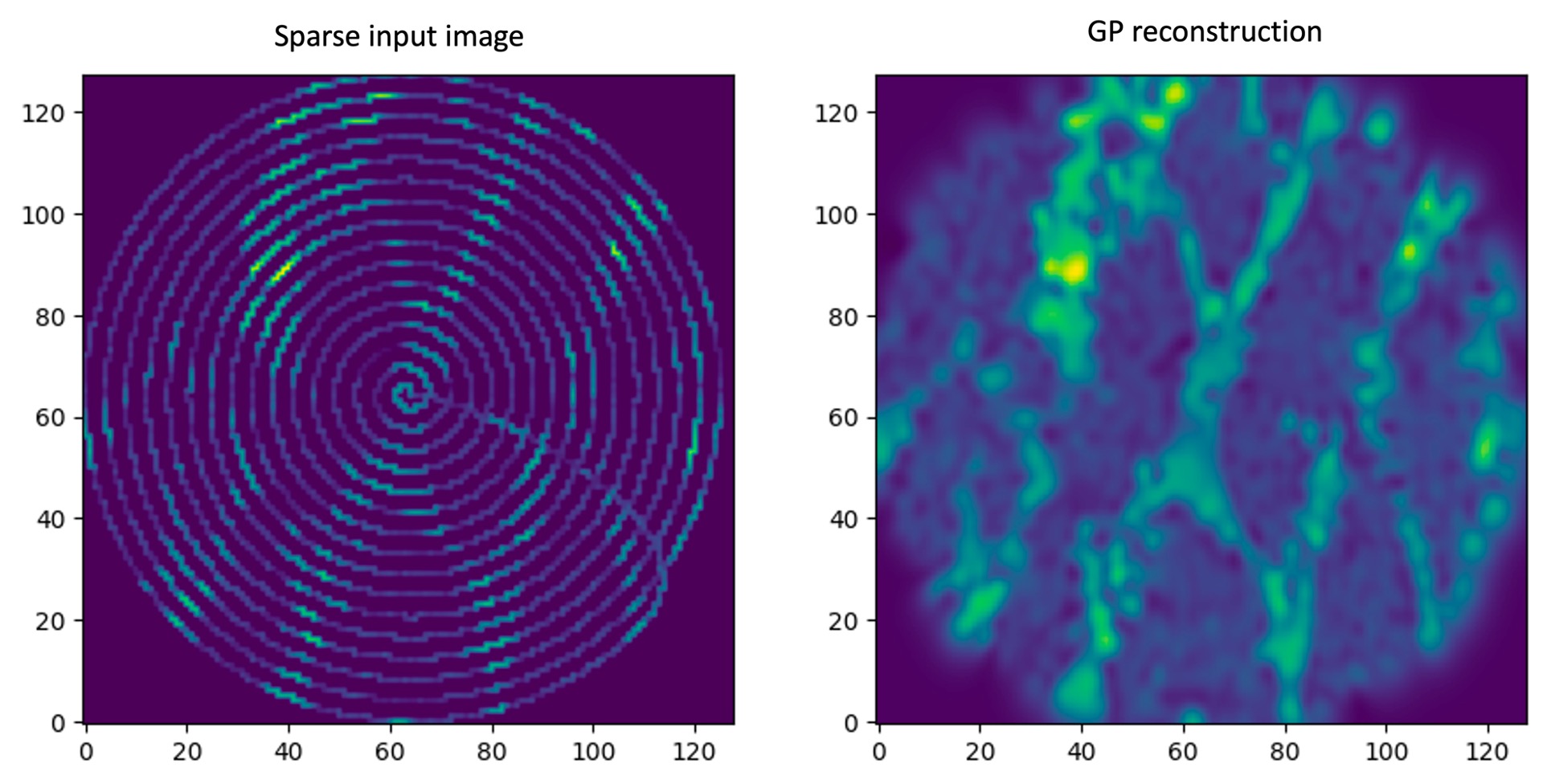 Finally, for larger images or hyperspecteral data, one can use the [inducing inputs](https://www.jmlr.org/papers/volume6/quinonero-candela05a/quinonero-candela05a.pdf) approximation to GP, which is also available in GPax. See the full example [here](https://colab.research.google.com/github/ziatdinovmax/gpax/blob/main/examples/gpax_viGP.ipynb). ### Structured GP [](https://colab.research.google.com/github/ziatdinovmax/gpax/blob/main/examples/GP_sGP.ipynb) The limitation of the standard GP is that it does not usually allow for the incorporation of prior domain knowledge and can be biased toward a trivial interpolative solution. Recently, we [introduced](https://arxiv.org/abs/2108.10280) a structured Gaussian Process (sGP), where a classical GP is augmented by a structured probabilistic model of the expected system’s behavior. This approach allows us to [balance](https://towardsdatascience.com/unknown-knowns-bayesian-inference-and-structured-gaussian-processes-why-domain-scientists-know-4659b7e924a4) the flexibility of the non-parametric GP approach with a rigid structure of prior (physical) knowledge encoded into the parametric model. Implementation-wise, we substitute a constant/zero prior mean function in GP with a probabilistic model of the expected system's behavior. For example, if we have prior knowledge that our objective function has a discontinuous 'phase transition', and a power law-like behavior before and after this transition, we may express it using a simple piecewise function ```python3 import jax.numpy as jnp def piecewise(x: jnp.ndarray, params: Dict[str, float]) -> jnp.ndarray: """Power-law behavior before and after the transition""" return jnp.piecewise( x, [x < params["t"], x >= params["t"]], [lambda x: x**params["beta1"], lambda x: x**params["beta2"]]) ``` where ```jnp``` corresponds to jax.numpy module. This function is deterministic. To make it probabilistic, we put priors over its parameters with the help of [NumPyro](https://github.com/pyro-ppl/numpyro) ```python3 import numpyro from numpyro import distributions def piecewise_priors(): # Sample model parameters t = numpyro.sample("t", distributions.Uniform(0.5, 2.5)) beta1 = numpyro.sample("beta1", distributions.Normal(3, 1)) beta2 = numpyro.sample("beta2", distributions.Normal(3, 1)) # Return sampled parameters as a dictionary return {"t": t, "beta1": beta1, "beta2": beta2} ``` Finally, we train the sGP model and make predictions on new data in the almost exact same way we did for vanilla GP. The only difference is that we pass our structured probabilistic model as two new arguments (the piecewise function and the corresponding priors over its parameters) when initializing GP. ```python3 # Get random number generator keys rng_key, rng_key_predict = gpax.utils.get_keys() # initialize structured GP model sgp_model = gpax.ExactGP(1, kernel='Matern', mean_fn=piecewise, mean_fn_prior=piecewise_priors) # Run MCMC to obtain posterior samples sgp_model.fit(rng_key, X, y) # Get GP prediction on new/test data posterior_mean, f_samples = sgp_model.predict(rng_key_predict, X_test) ``` 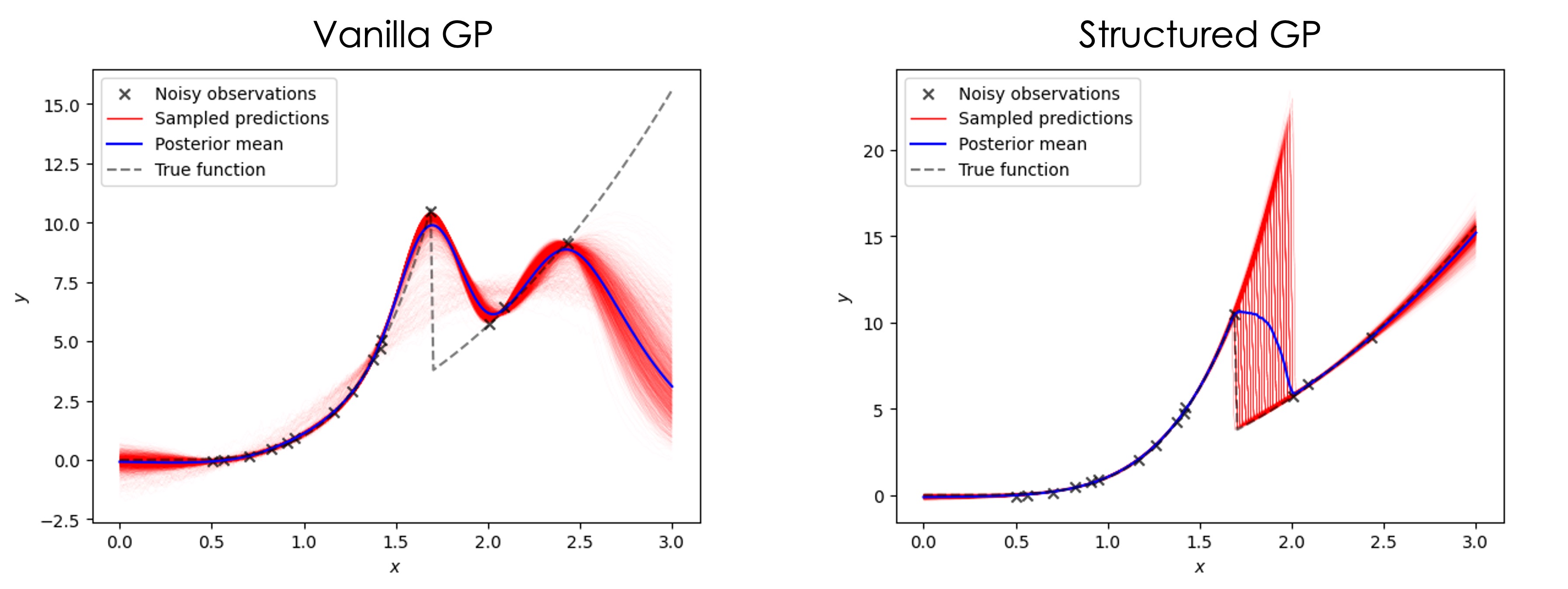 Structured GP is usually better at extrapolation and provides more reasonable uncertainty estimates. The probabilistic model in structured GP reflects our prior knowledge about the system, but it does not have to be precise, that is, the model can have a different functional form, as long as it captures general or partial trends in the data. The full example including the active learning part is available [here](https://colab.research.google.com/github/ziatdinovmax/gpax/blob/main/examples/GP_sGP.ipynb). ### Active learning and Bayesian optimization [](https://colab.research.google.com/github/ziatdinovmax/gpax/blob/main/examples/gpax_GPBO.ipynb) Both GP and sGP can be used for active learning to reconstruct the entire data distribution from sparse observations or to localize regions of the parameter space where a particular physical behavior is maximized or minimized with as few measurements as possible (the latter is usually referred to as [Bayesian optimization](https://ieeexplore.ieee.org/abstract/document/7352306)). ```python3 # Train a GP model (it can be sGP or vanilla GP) gp_model.fit(rng_key, X_measured, y_measured) # A # Compute the upper confidence bound (UCB) acquisition function to derive the next measurement point acq = gpax.acquisition.UCB(rng_key_predict, gp_model, X_unmeasured, beta=4, maximize=False, noiseless=True) # B next_point_idx = acq.argmax() # C next_point = X_unmeasured[next_point_idx] # D # Perform measurement in next_point, update measured & unmeasured data arrays, and re-run steps A-D. ``` In the figure below we illustrate the connection between the (s)GP posterior predictive distribution and the acquisition function used to derive the next measurement points. Here, the posterior mean values indicate that the minimum of a "black box" function describing a behavior of interest is around $x=0.7$. At the same time, there is a large dispersion in the samples from the posterior predictive distribution between $x=-0.5$ and $x=0.5$, resulting in high uncertainty in that region. The acquisition function is computed as a function of both predictive mean and uncertainty and its maximum corresponds to the next measurement point in the active learning and Bayesian optimization. Here, after taking into account the uncertainty in the prediction, the UCB acquisition function suggests exploring a point at x≈0 where potentially a true minimum is located. See full example [here](https://colab.research.google.com/github/ziatdinovmax/gpax/blob/main/examples/gpax_GPBO.ipynb). <img src="https://github.com/ziatdinovmax/gpax/assets/34245227/24f641fb-5959-4780-8d0e-edf62bd0a32b"> ### Theory-informed data reconstruction and Bayesian optimization [](https://colab.research.google.com/github/ziatdinovmax/gpax/blob/main/examples/GPax_MultiTaskGP_BO.ipynb) Sometimes when theoretical simulations are available before the experiment, they can be used to guide the measurements or simply reconstruct sparse data via a multi-task/fidelity Gaussian process. This can be used as an alternative solution to a structured Gaussian process in situations where a mean function is too costly to compute at each step or it is expressed through some complex program that is not fully differentiable. The overall scheme is the same, but now our GP model is a MultitaskGP: ```python3 key1, key2 = gpax.utils.get_keys(1) gp_model = gpax.MultiTaskGP( input_dim=1, data_kernel='Matern', # standard GP parameters shared_input_space=False, # different tasks/fidelities have different numbers of observations num_latents=2, rank=2, # parameters of multi-task GP ) model.fit(key1, X, y, num_warmup=500, num_samples=500) ``` Note that X has (N, D+1) dimensions where the last column contains task/fidelity indices for each observation. We can then use the trained model to make a prediction for partially observed data: ```python3 # Create a set of inputs for the task/fidelity 2 X_unmeasured2 = np.column_stack((X_full_range, np.ones_like(X_full_range))) # Make a prediction with the trained model posterior_mean2, f_samples2 = model.predict(key2, X_unmeasured2, noiseless=True) ``` 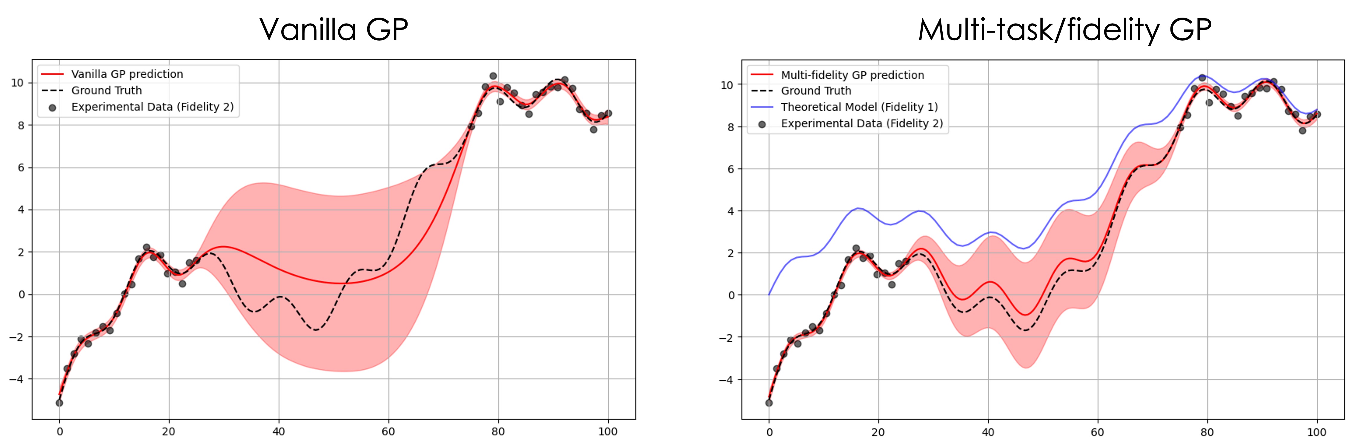 The full example including Bayesian optimization is available [here](https://colab.research.google.com/github/ziatdinovmax/gpax/blob/main/examples/GPax_MultiTaskGP_BO.ipynb) ### Hypothesis learning [](https://colab.research.google.com/github/ziatdinovmax/gpax/blob/main/examples/gpax_hypo.ipynb) The structured GP can also be used for hypothesis learning in automated experiments. The [hypothesis learning](https://arxiv.org/abs/2112.06649) is based on the idea that in active learning, the correct model of the system’s behavior leads to a faster decrease in the overall Bayesian uncertainty about the system under study. In the hypothesis learning setup, probabilistic models of the possible system’s behaviors (hypotheses) are wrapped into structured GPs, and a basic reinforcement learning policy is used to select a correct model from several competing hypotheses. The example of hypothesis learning on toy data is available [here](https://colab.research.google.com/github/ziatdinovmax/gpax/blob/main/examples/gpax_hypo.ipynb). <img src="https://user-images.githubusercontent.com/34245227/167936394-52f5ffd5-a47c-425d-b8a7-0727938dfab2.gif"> ### Deep kernel learning [](https://colab.research.google.com/github/ziatdinovmax/gpax/blob/main/examples/gpax_viDKL_plasmons.ipynb) [Deep kernel learning (DKL)](https://arxiv.org/abs/1511.02222) can be understood as a hybrid of deep neural network (DNN) and GP. The DNN serves as a feature extractor that allows reducing the complex high-dimensional features to low-dimensional descriptors on which a standard GP kernel operates. The parameters of DNN and of GP kernel are inferred jointly in an end-to-end fashion. Practically, the DKL training inputs are usually patches from an (easy-to-acquire) structural image, and training targets represent a physical property of interest derived from the (hard-to-acquire) spectra measured in those patches. The DKL output on the new inputs (image patches for which there are no measured spectra) is the expected property value and associated uncertainty, which can be used to derive the next measurement point in the automated experiment. GPax package has the fully Bayesian DKL (weights of neural network and GP hyperparameters are inferred using Hamiltonian Monte Carlo) and the Variational Inference approximation of DKL, viDKL. The fully Bayesian DKL can provide an asymptotically exact solution but is too slow for most automated experiments. Hence, for the latter, one may use the viDKL ```python3 import gpax # Get random number generator keys for training and prediction rng_key, rng_key_predict = gpax.utils.get_keys() # Obtain/update DKL posterior; input data dimensions are (n, h*w*c) dkl = gpax.viDKL(input_dim=X.shape[-1], z_dim=2, kernel='RBF') # A dkl.fit(rng_key, X_train, y_train, num_steps=100, step_size=0.05) # B # Compute UCB acquisition function obj = gpax.acquisition.UCB(rng_key_predict, dkl, X_unmeasured, maximize=True) # C # Select next point to measure (assuming grid data) next_point_idx = obj.argmax() # D # Perform measurement in next_point_idx, update measured & unmeasured data arrays, and re-run steps A-D. ``` Below we show a result of a simple DKL-based search for regions of the nano-plasmonic array that [host edge plasmons](https://arxiv.org/abs/2108.03290). The full example is available [here](https://colab.research.google.com/github/ziatdinovmax/gpax/blob/main/examples/gpax_viDKL_plasmons.ipynb). <img src="https://user-images.githubusercontent.com/34245227/160270568-147fa21b-91f3-48b8-8dd2-c33eb4b497b4.png"> Note that in viDKL, we use a simple MLP as a default feature extractor. However, you can easily write a custom DNN using [haiku](https://github.com/deepmind/dm-haiku) and pass it to the viDKL initializer ```python3 import haiku as hk class ConvNet(hk.Module): def __init__(self, embedim=2): super().__init__() self._embedim = embedim def __call__(self, x): x = hk.Conv2D(32, 3)(x) x = jax.nn.relu(x) x = hk.MaxPool(2, 2, 'SAME')(x) x = hk.Conv2D(64, 3)(x) x = jax.nn.relu(x) x = hk.Flatten()(x) x = hk.Linear(self._embedim)(x) return x dkl = gpax.viDKL(X.shape[1:], 2, kernel='RBF', nn=ConvNet) # input data dimensions are (n,h,w,c) dkl.fit(rng_key, X_train, y_train, num_steps=100, step_size=0.05) obj = gpax.acquisition.UCB(rng_key_predict, dkl, X_unmeasured, maximize=True) next_point_idx = obj.argmax() ``` ## Installation If you would like to utilize a GPU acceleration, follow these [instructions](https://github.com/google/jax#installation) to install JAX with a GPU support. Then, install GPax using pip. We recommend installing the latest stable deployment from PyPI using ```bash pip install gpax ``` Otherwise, if you are confident in what's on the `main` branch of GPax, you can also install directly from the GitHub repository: ```bash pip install git+https://github.com/ziatdinovmax/gpax ``` If you are a Windows user, we recommend to use the Windows Subsystem for Linux (WSL2), which comes free on Windows 10 and 11. ## Cite us If you use GPax in your work, please consider citing our papers: ``` @article{ziatdinov2021physics, title={Physics makes the difference: Bayesian optimization and active learning via augmented Gaussian process}, author={Ziatdinov, Maxim and Ghosh, Ayana and Kalinin, Sergei V}, journal={arXiv preprint arXiv:2108.10280}, year={2021} } @article{ziatdinov2021hypothesis, title={Hypothesis learning in an automated experiment: application to combinatorial materials libraries}, author={Ziatdinov, Maxim and Liu, Yongtao and Morozovska, Anna N and Eliseev, Eugene A and Zhang, Xiaohang and Takeuchi, Ichiro and Kalinin, Sergei V}, journal={arXiv preprint arXiv:2112.06649}, year={2021} } ``` ## Funding acknowledgment This work was supported by the U.S. Department of Energy, Office of Science, Basic Energy Sciences Program.